決定木(Decision Tree)とランダムフォレスト(Random Forest)について。
【目次】
決定木(Decision Tree)
分類問題、回帰問題の両方に対応でき、それぞれ「分類木」「回帰木」と呼ばれる。
決定木は、分割前後の不純度の差(情報利得)が最大になるように学習する。
Python 基本コード
from sklearn.tree import DecisionTreeClassifier
mod1 = RandomForestClassifier(criterion = "gini", max_depth = i_integer)
mod1.fit(X_train, y_train)

= 特徴量(説明変数)

= 親ノード、左右の子ノードの不純度

= 親ノード、左右の子ノードのサンプル数
情報利得は分割前後の不純度(Impurity Criterion)の差である。
複数分類が混合する分割前データから各分類をきれいに分離できるほど分割前後の不純度の差は大きくなる。このことから、情報利得の最大化が目的関数となる。
次の図は、分割方法AとBを比較したものである。この例では、分割方法Bの方が分割後の不純度が小さいので情報利得が大きくなる。したがって、情報利得を最大化できる分割方法Bが選択される。

不純度(Impurity Criterion)
Python scikit-learn 0.24.2 では、不純度の評価指標としてジニ係数(Gini Index)とエントロピー(Entropy)が実装されている。
ジニ係数を使ったアルゴリズムにはCART(Classification And Regression Trees)、エントロピーを使ったアルゴリズムにはC4.5がある。
エントロピー(Entropy)
ジニ係数(Gini Index)
分析例
次のサンプルデータで手順を追ってみる。
目的変数は★〇△の3分類。特徴量はX1、X2、X3の3つ。

サンプルサイズ10個、★5個、〇3個、△2個なので、不純度(初期値)は:
これを特徴量X1(A or notA)で分割すると次の通り:

よって情報利得は:
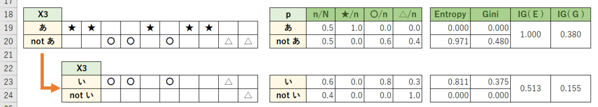
同じように、特徴量X2(1 or 2)、X3("あ" or not"あ")でも計算してみる:
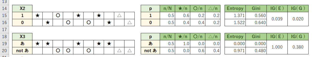
ジニ係数で話を進めると、情報利得は X3 = 0.380 が最大のため、特徴量X3で分割する。
python コード
import pandas as pd
from sklearn.tree import DecisionTreeClassifier, plot_tree
import matplotlib.pyplot as plt
df = pd.DataFrame({"y": ["★","★","☆","☆","★","☆","★","★","△","△"]
,"X1": ["A","A","A","B","B","B","B","C","C","B"]
,"X2": [1,0,1,0,1,0,1,0,1,0]
,"X3": ["あ","あ","い","い","あ","い","あ","あ","い","う"]})
df = pd.get_dummies(df, columns=["X1", "X3"])
def DecisionTree(lst, criterion1, max_depth1):
clf = DecisionTreeClassifier(criterion=criterion1, max_depth=max_depth1)
clf.fit(X=df[lst], y=df["y"])
plot_tree(clf, filled=True, fontsize=12, feature_names=lst)
plt.figure(figsize=(15,5))
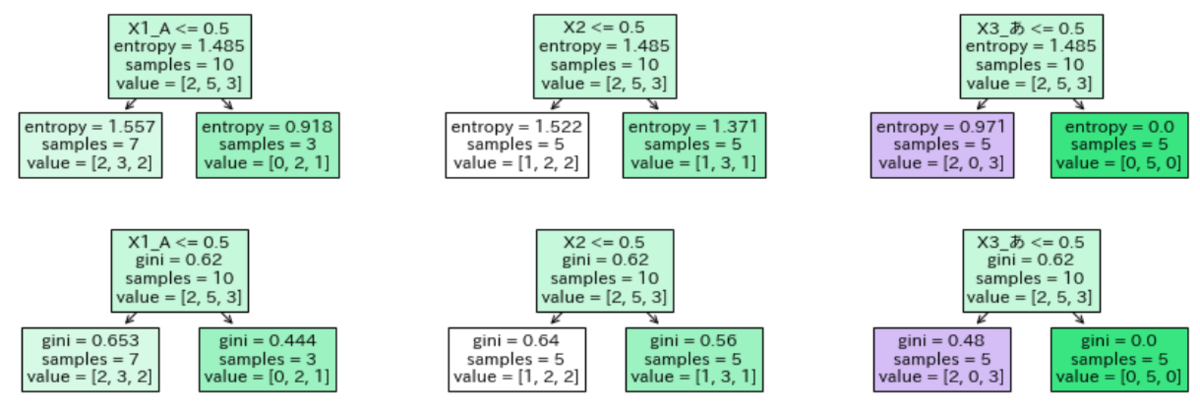
plt.subplot(2, 3, 1); DecisionTree(lst=["X1_A"], criterion1="entropy", max_depth1=1)
plt.subplot(2, 3, 2); DecisionTree(lst=["X2"], criterion1="entropy", max_depth1=1)
plt.subplot(2, 3, 3); DecisionTree(lst=["X3_あ"], criterion1="entropy", max_depth1=1)
plt.subplot(2, 3, 4); DecisionTree(lst=["X1_A"], criterion1="gini", max_depth1=1)
plt.subplot(2, 3, 5); DecisionTree(lst=["X2"], criterion1="gini", max_depth1=1)
plt.subplot(2, 3, 6); DecisionTree(lst=["X3_あ"], criterion1="gini", max_depth1=1)
plt.show()
勉強がてら更にもう1深度分割してみる。
plt.figure(figsize=(10,5))
plt.subplot(1, 2, 1); DecisionTree(lst=["X1_A","X1_B","X2","X3_あ","X3_い"], criterion1="gini", max_depth1=2)
plt.subplot(1, 2, 2); DecisionTree(lst=["X1_A","X1_B","X2","X3_あ","X3_い"], criterion1="entropy", max_depth1=2)
plt.show()
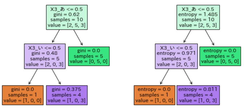
今回のサンプルデータでは「X3="あ" or not"あ"」→「X3="い" or not"い"」の分岐が良いようであった。
決定木の応用
ランダムフォレスト、XGboost及びLightGBMなど良く耳にする手法は、決定木を学習器としたアンサンブル学習(バギング、ブースティング等)であり、高い精度を持つ。

※本記事ではランダムフォレストについて触れたい。XGboost、LightGBMは別の記事で。
ランダムフォレスト(Random Forest)
ランダムフォレストは決定木と同様に分類問題、回帰問題の両方に対応できる。
決定木を並列で実行し、最終結果を得るバギング(アンサンブル学習の1つ)という方法をとる。
Python 基本コード
from sklearn.ensemble import RandomForestClassifier
mod1 = RandomForestClassifier(n_estimators = 100
                              ,criterion = "gini"
                              ,max_depth = i_integer
                              ,max_features = "auto"
                              ,bootstrap = True
                              ,random_state = 1)
ランダムフォレストの流れ
ランダムフォレストの基本的な流れは次の通り。
Bootstrap samplingにて、訓練データからサンプルサイズnの小標本を生成する。Samplingの重複は許容される(例:Aさんの同一データが複数回抽出されてもOK)。
引数:bootstrap。デフォルトはTrue。
上記1の小標本について、学習に用いる特徴量(説明変数)をランダムにm個決める(例:身長、体重、脈拍、血圧の特徴量から身長、脈拍のみを学習に用いる)。
引数:max_features={"auto", "sqrt", "log2"}。デフォルトは"auto"。"auto"では√m個の特徴量が指定される。
上記1,2で決定木をk個つくり学習する。※上記1のみならバギングツリー、上記1,2両方ならランダムフォレスト。
分類アルゴリズムはCART(ジニ係数)とC4.5(エントロピー)がある。
引数:n_estimators。作成する決定木の数を指定。デフォルトは100。
引数:criterion={“gini”, “entropy”}。デフォルトは"gini"(ジニ係数)。
引数:max_depth。決定木の深さを指定。デフォルトはNone。簡易決定木のため、通常の決定木より小さい値にすると良い。
上記3の決定木を使ってテストデータで予測する。
各決定木の結果を多数決(分類問題)や平均化(回帰問題)して最終結果を出す。
評価指標を用いてモデルを評価する。
wineデータを使った分析例
3分類のワインデータを決定木とランダムフォレストで分類してみる。
※データ詳細は以下。
sklearn.datasets.load_wine — scikit-learn 0.24.2 documentation
ランダムサーチでハイパーパラメータを調整し、得られた結果を混同行列やF1スコアで評価する。
import pandas as pd
import numpy as np
from scipy import stats
from sklearn import datasets, model_selection
from sklearn.tree import DecisionTreeClassifier
from sklearn.ensemble import RandomForestClassifier
from sklearn.metrics import classification_report, confusion_matrix
ROW = datasets.load_wine()
ADS = pd.DataFrame(ROW.data, columns=ROW.feature_names).assign(target=np.array(ROW.target))
X_train, X_test, y_train, y_test = model_selection.train_test_split(
ADS[ROW.feature_names], ADS["target"], test_size=0.3, random_state=1)
modfnc1 = [DecisionTreeClassifier(), RandomForestClassifier()]
prm1 = [{"max_depth": stats.randint(1,6)
,"criterion":["gini","entropy"]
,"random_state":[1]}
,{"n_estimators": stats.randint(10,201)
,"max_depth": stats.randint(1,6)
,"criterion":["gini","entropy"]
,"max_features":["auto", "sqrt", "log2"]
,"random_state":[1]}]
for modfnc1, prm1 in zip(modfnc1, prm1):
clf = model_selection.RandomizedSearchCV(modfnc1, prm1)
clf.fit(X_train, y_train)
y_pred1 = clf.predict(X_test)
print(clf.best_estimator_)
print(confusion_matrix(y_test, y_pred1))
print(classification_report(y_test, y_pred1))
print()
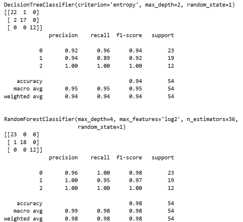
今回の結果では、ランダムフォレストの方がF1スコア等が高く良好のようだった。
参考
1.10. Decision Trees — scikit-learn 0.24.2 documentation
Understanding Decision Trees for Classification (Python) | by Michael Galarnyk | Towards Data Science
決定木分析のパラメータ解説 – S-Analysis